library(magrittr)
library(car)
library(flextable)
library(readr)
library(readxl)
library(purrr)
library(ggplot2)
library(dplyr)
library(stats)
library(tseries)
library(zoo)
library(dynlm)
library(forecast)
library(strucchange)
library(lubridate)
library(dLagM)Experiment 3
load packages
1.
Read the data.
quarterly <- read_xlsx("data/us_macro_quarterly.xlsx")
quarterly$...1 <- as.yearqtr(quarterly$...1, "%Y:%q")

quarterly <- quarterly %>% filter(`...1` >= as.yearqtr("1963 Q1") & `...1` <= as.yearqtr("2012 Q4"))
a.
i.
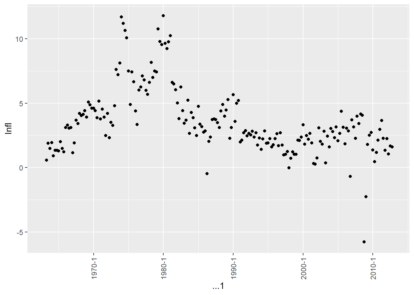
The inflation rate Infl is measured in percentage per quarter. It is calculated as the log difference of PCEP multiplied by 400. Since PCEP is an index, its log difference approximates the percentage change. Multiplying by 400 annualizing this quarterly change into a percentage per year.
PCEPs <- quarterly %>% select(PCECTPI) %>% pull()
infl <- diff(log(PCEPs)) * 400
quarterly <- quarterly %>% mutate(Infl = c(NA, infl))
ii.
Based on the plot, Infl does not appear to have a stochastic trend. It fluctuates around a relatively stable mean over time, rather than exhibiting a consistent upward or downward trend. While there are periods of higher or lower inflation, it tends to revert toward the long-run average over time. This suggests Infl is a stationary series.
b.
i.
spec_infl <- quarterly %>%
  select("Infl") %>%
  pull()
delta <- diff(spec_infl)
acf(delta[2:length(delta)], plot = FALSE, lag = 4)
Autocorrelations of series 'delta[2:length(delta)]', by lag

     0      1      2      3      4
 1.000 -0.252 -0.183  0.133 -0.094
ii.
ts.plot(delta)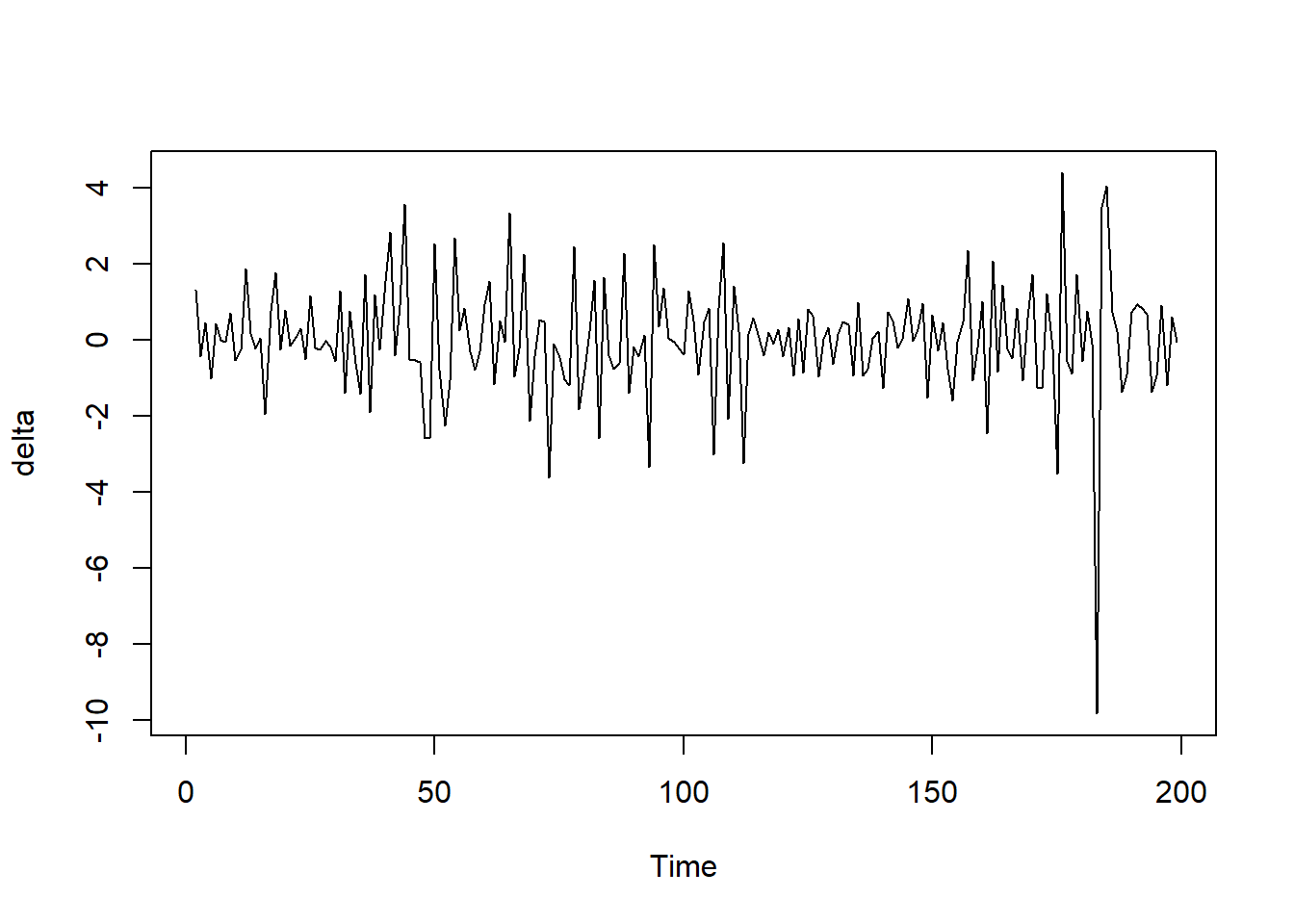
The negative autocorrelation shows that inflation rates tend to reverse direction from quarter to quarter, rather than continue in the same direction. So a quarter with high inflation is more likely to be followed by a quarter with lower inflation, and vice versa. This results in the choppy, oscillating pattern seen in the plot. So in summary, the jagged, choppy plot of delta_pcep matches what we would expect given the negative first autocorrelation, indicating the inflation rate tends to reverse course from quarter to quarter. The plot and autocorrelation results confirm one another.
c.
i.
ar_quarter <- arima(delta, order = c(1, 0, 0))
print(ar_quarter)
Call:
arima(x = delta, order = c(1, 0, 0))

Coefficients:
          ar1  intercept
      -0.2514     0.0040
s.e.   0.0687     0.0827

sigma^2 estimated as 2.116:  log likelihood = -355.19,  aic = 716.39
The coefficient is statistically significant. This indicates that knowing the change in inflation this quarter helps predict the change in inflation next quarter
ii.
ar2_quarter <- arima(delta, order = c(2, 0, 0))
print(ar2_quarter)
Call:
arima(x = delta, order = c(2, 0, 0))

Coefficients:
          ar1      ar2  intercept
      -0.3176  -0.2619     0.0028
s.e.   0.0686   0.0683     0.0633

sigma^2 estimated as 1.969:  log likelihood = -348.12,  aic = 704.23
aic of AR(2) model is smaller than the AR(1) model, so AR(2) model is better.
iii.
ar_aic <- function(x, p) {
  arima(x, order = c(p, 0, 0)) %>% .$aic
}
ar_bic <- function(x, p) {
  arima(x, order = c(p, 0, 0)) %>% AIC(k = log(length(x)))
}
aics <- c()
bics <- c()
for (i in 0:8) {
  aics <- c(aics, ar_aic(delta, i))
  bics <- c(bics, ar_bic(delta, i))
}
bics
[1] 733.9226 726.2685 717.4061 722.6805 725.5250 728.3784 732.0999 737.2160
[9] 742.3509aics[1] 727.3360 716.3886 704.2328 706.2139 705.7652 705.3253 705.7534 707.5763
[9] 709.4178From the results, lag length of 2 is chosen both by BIC and AIC.
iv.
predict(ar2_quarter, 1) %>% .$pred %>% as.numeric()[1] -0.1379599v.
ar2_infl <- arima(infl, order = c(2, 0, 0))
predict(ar2_infl, 1) %>% .$pred %>% as.numeric()
[1] 1.875945d.
i.
adf.test(delta[2:length(delta)], k = 2)
    Augmented Dickey-Fuller Test

data:  delta[2:length(delta)]
Dickey-Fuller = -9.8603, Lag order = 2, p-value = 0.01
alternative hypothesis: stationary
ii.
There is no time trend. So the first one is better
iii.
More or less lags are not necessary, because from the BIC and AIC, number of lags has been chosen to be 2. More lags will make it bias and fewer lags will enlarge the variance.
iv.
adf.test(infl, k = 2)
    Augmented Dickey-Fuller Test

data:  infl
Dickey-Fuller = -3.2971, Lag order = 2, p-value = 0.0733
alternative hypothesis: stationary
The DF-stat is bigger than the 5% critical value, but smaller than the 10% critical, so we are 90% sure that the AR model for Infl contains a unit root.
e.
没搞懂。。。这里跑不出来,折腾一天,我甚至觉得题有问题,弃了弃了
quarterly$delta <- c(NA, quarterly %>%
  select("Infl") %>%
  pull() %>%
  diff())

trimming <- 0.15 * nrow(quarterly) %>% round()
df <- quarterly[trimming:(nrow(quarterly)-trimming),]
tau <- seq(as.numeric(df$...1[1]), as.numeric(last(df$...1)), 0.25)
Fstats <- c()

delta_infl <- quarterly[trimming:(nrow(quarterly)-trimming),] %>%
  select("delta") %>%
  pull()

for(i in 1:length(tau)) {
  D <- as.numeric((df$...1-df$...1[1]) >= tau[i]-1970)
  fit <- dynlm(
    delta_infl ~ L(delta_infl, 1) + L(delta_infl, 2) +
      D + D * L(delta_infl) + D * L(delta_infl, 2),
    data = df
  )
  linearHypothesis(fit,
    "D=0",
    vcov. = sandwich
  )$F[2]

}
f.
i.
x <- quarterly %>% filter(...1 <= as.yearqtr("2012 Q3"))
predicts <- c()
while (last(x$...1) >= as.yearqtr("2002 Q4")) {
  pre <- arima(diff(x$Infl), order = c(2, 0, 0)) %>%
    predict(1) %>%
    .$pred %>% as.numeric()
  predicts <- c(predicts, pre)
  x <- x[1:nrow(x)-1,]
}
predicts <- rev(predicts)

real <- quarterly %>%
  filter(...1 <= as.yearqtr("2012 Q4") & ...1 >= as.yearqtr("2002 Q4")) %>%
  select(Infl) %>%
  pull() %>% diff()

mean(real-predicts)
[1] -0.02157171tibble(real, predicts) %>% ggplot(aes(x = 1:40, y = c(real, predicts))) + geom_line(aes(y = real, color = "real")) + geom_line(aes(y = predicts, color = "predicts"))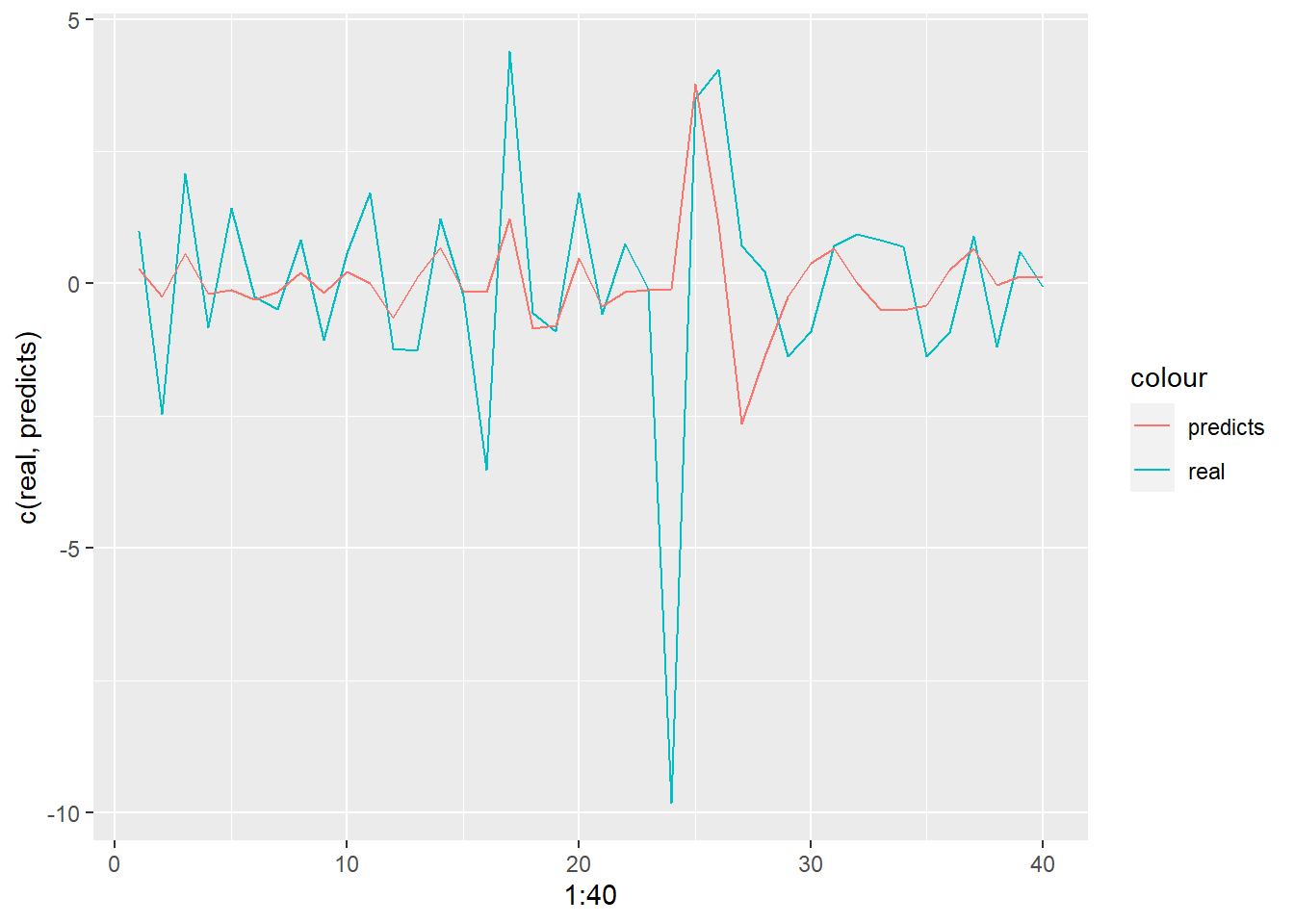
ii.
The forecast errors mean value is close to 0, so it is unbiased.
iii.
sqrt(sum((real-predicts)^2) / length(real))[1] 2.057148predicts2 <- quarterly %>%
filter(...1 >= as.yearqtr("1963 Q1") & ...1 <= as.yearqtr("2002 Q4")) %>%
select("Infl") %>%
pull() %>%
diff() %>%
arima(order = c(2, 0, 0)) %>%
predict(40) %>% .$pred %>% as.numeric()
sqrt(sum((real-predicts2)^2) / length(real))[1] 2.217931From the RMSFE, the two forecasts are consistent.
iv.
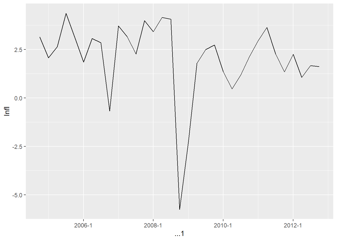
From above gas price data, we can see the price fell sharply in 2008 Q4. This sharp decline in oil prices could be one of the reasons why inflation fell so much in 2008:Q4.
2.
a.
monthly <- read_xlsx("data/us_macro_monthly.xlsx")
monthly$...1 <- fast_strptime(monthly$...1, format = "%Y:%m") %>% as.yearmon()
ip_growth <- 100 * diff(log(monthly$INDPRO))

monthly <- monthly %>%
  mutate(ip_growth = c(NA, ip_growth))

monthly %>%
  filter(...1 <= as.yearmon("2012-12") & ...1 >= 1960-01) %>%
  select("ip_growth") %>%
  pull() %>% {
    print(mean(.))
    print(sd(.))
  }
[1] 0.2335855
[1] 0.8306868So the mean value is 0.234, and the standard deviation is 0.831. We took the monthly log difference, so ip_growth is expressed as a percent per month.
b.
monthly %>% ggplot(aes(y = `0_T`, x = ...1)) + geom_point()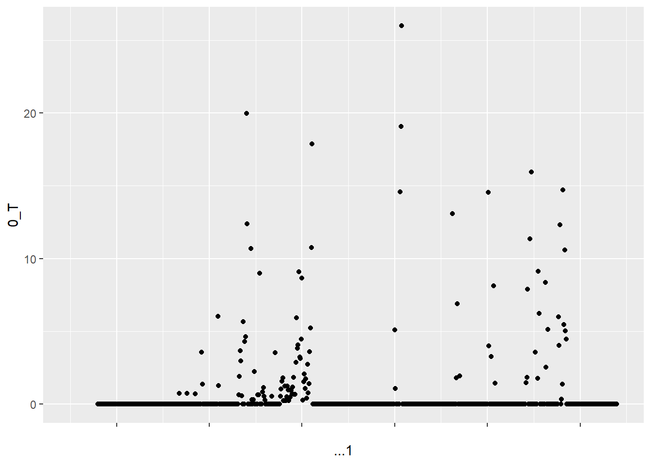
0_T is defined as the greater of zero or the percentage point difference between oil prices at date t and their maximum value during the past 3 years. This means that if oil prices at date t are lower than their maximum value during the past 3 years, then 0_T will be equal to zero. This is why so many values of 0_T are equal to zero. The values of 0_T cannot be negative because it is defined as the greater of zero or the percentage point difference between oil prices at date t and their maximum value during the past 3 years.
c.
data <- monthly %>%
  mutate(T = monthly$`0_T`) %>%
  select(ip_growth, T)
data_with_lags <- data %>%
  mutate(
    lag1_T = lag(T, 1),
    lag2_T = lag(T, 2),
    lag3_T = lag(T, 3),
    lag4_T = lag(T, 4),
    lag5_T = lag(T, 5),
    lag6_T = lag(T, 6),
    lag7_T = lag(T, 7),
    lag8_T = lag(T, 8),
    lag9_T = lag(T, 9),
    lag10_T = lag(T, 10),
    lag11_T = lag(T, 11),
    lag12_T = lag(T, 12),
    lag13_T = lag(T, 13),
    lag14_T = lag(T, 14),
    lag15_T = lag(T, 15),
    lag16_T = lag(T, 16),
    lag17_T = lag(T, 17),
    lag18_T = lag(T, 18)
  ) %>%
  na.omit()
distributed_lag_model <- dynlm(
  ip_growth ~ T + lag1_T + lag2_T + lag3_T + lag4_T + lag5_T + lag6_T + lag7_T + lag8_T + lag9_T + lag10_T + lag11_T + lag12_T + lag13_T + lag14_T + lag15_T + lag16_T + lag17_T + lag18_T,
  data = data_with_lags
)
summary(distributed_lag_model)
Time series regression with "numeric" data:
Start = 1, End = 654

Call:
dynlm(formula = ip_growth ~ T + lag1_T + lag2_T + lag3_T + lag4_T +
    lag5_T + lag6_T + lag7_T + lag8_T + lag9_T + lag10_T + lag11_T +
    lag12_T + lag13_T + lag14_T + lag15_T + lag16_T + lag17_T +
    lag18_T, data = data_with_lags)

Residuals:
    Min      1Q  Median      3Q     Max
-3.8151 -0.4078  0.0097  0.3848  5.6295

Coefficients:
              Estimate Std. Error t value Pr(>|t|)
(Intercept)  0.3683933  0.0366821  10.043   <2e-16 ***
T            0.0067550  0.0129314   0.522   0.6016
lag1_T      -0.0201563  0.0137662  -1.464   0.1436
lag2_T      -0.0102141  0.0138368  -0.738   0.4607
lag3_T      -0.0061015  0.0138735  -0.440   0.6602
lag4_T      -0.0073852  0.0138773  -0.532   0.5948
lag5_T      -0.0103567  0.0138889  -0.746   0.4561
lag6_T      -0.0311658  0.0139014  -2.242   0.0253 *
lag7_T      -0.0009245  0.0138994  -0.067   0.9470
lag8_T       0.0058652  0.0138985   0.422   0.6732
lag9_T      -0.0187055  0.0139159  -1.344   0.1794
lag10_T     -0.0433425  0.0138985  -3.119   0.0019 **
lag11_T     -0.0351425  0.0138994  -2.528   0.0117 *
lag12_T     -0.0005823  0.0139014  -0.042   0.9666
lag13_T     -0.0150695  0.0138889  -1.085   0.2783
lag14_T     -0.0119535  0.0138773  -0.861   0.3894
lag15_T     -0.0165019  0.0138735  -1.189   0.2347
lag16_T     -0.0036165  0.0138368  -0.261   0.7939
lag17_T      0.0098934  0.0137662   0.719   0.4726
lag18_T      0.0087075  0.0129314   0.673   0.5010
---
Signif. codes:  0 '***' 0.001 '**' 0.01 '*' 0.05 '.' 0.1 ' ' 1

Residual standard error: 0.7778 on 634 degrees of freedom
Multiple R-squared:  0.1212,    Adjusted R-squared:  0.0949
F-statistic: 4.604 on 19 and 634 DF,  p-value: 5.574e-10
T <- nrow(data_with_lags)
m <- floor(T^(1/3))Using rule of thumb, the m is 8
d.
linearHypothesis(
  distributed_lag_model,
  c("T=0", "lag1_T=0", "lag2_T=0", "lag3_T=0", "lag4_T=0", "lag5_T=0", "lag6_T=0", "lag7_T=0", "lag8_T=0", "lag9_T=0", "lag10_T=0", "lag11_T=0", "lag12_T=0", "lag13_T=0", "lag14_T=0", "lag15_T=0", "lag16_T=0", "lag17_T=0", "lag18_T=0")
)
Linear hypothesis test
Hypothesis:
T = 0
lag1_T = 0
lag2_T = 0
lag3_T = 0
lag4_T = 0
lag5_T = 0
lag6_T = 0
lag7_T = 0
lag8_T = 0
lag9_T = 0
lag10_T = 0
lag11_T = 0
lag12_T = 0
lag13_T = 0
lag14_T = 0
lag15_T = 0
lag16_T = 0
lag17_T = 0
lag18_T = 0
Model 1: restricted model
Model 2: ip_growth ~ T + lag1_T + lag2_T + lag3_T + lag4_T + lag5_T +
lag6_T + lag7_T + lag8_T + lag9_T + lag10_T + lag11_T + lag12_T +
lag13_T + lag14_T + lag15_T + lag16_T + lag17_T + lag18_T
Res.Df RSS Df Sum of Sq F Pr(>F)
1 653 436.48
2 634 383.56 19 52.918 4.6036 5.574e-10 ***
---
Signif. codes: 0 '***' 0.001 '**' 0.01 '*' 0.05 '.' 0.1 ' ' 1The result of F-stats shows that taken as a group, coefficients on 0_T are statistically significantly different from zero.
e.
# Calculate dynamic multipliers
dynamic_multipliers <- c(distributed_lag_model$coef[2:20])

# Calculate cumulative multipliers
cumulative_multipliers <- cumsum(dynamic_multipliers)

# Calculate 95% confidence intervals for dynamic multipliers
dynamic_ci <- confint(distributed_lag_model)[2:20,]

# Calculate 95% confidence intervals for cumulative multipliers
cumulative_ci <- apply(dynamic_ci, 2, cumsum)

# Create a data frame for plotting
plot_data <- data.frame(
  lag = 1:19,
  dynamic_multipliers = dynamic_multipliers,
  cumulative_multipliers = cumulative_multipliers,
  dynamic_ci_lower = dynamic_ci[, 1],
  dynamic_ci_upper = dynamic_ci[, 2],
  cumulative_ci_lower = cumulative_ci[, 1],
  cumulative_ci_upper = cumulative_ci[, 2]
)

# Plot dynamic multipliers and cumulative multipliers with 95% confidence intervals
ggplot(plot_data, aes(x = lag)) +
  geom_line(aes(y = dynamic_multipliers), color = "blue") +
  geom_ribbon(aes(ymin = dynamic_ci_lower, ymax = dynamic_ci_upper), alpha = 0.2, fill = "blue") +
  geom_line(aes(y = cumulative_multipliers), color = "red") +
  geom_ribbon(aes(ymin = cumulative_ci_lower, ymax = cumulative_ci_upper), alpha = 0.2, fill = "red") +
  labs(x = "Lag", y = "Multiplier", title = "Dynamic and Cumulative Multipliers with 95% Confidence Intervals") +
  theme_minimal()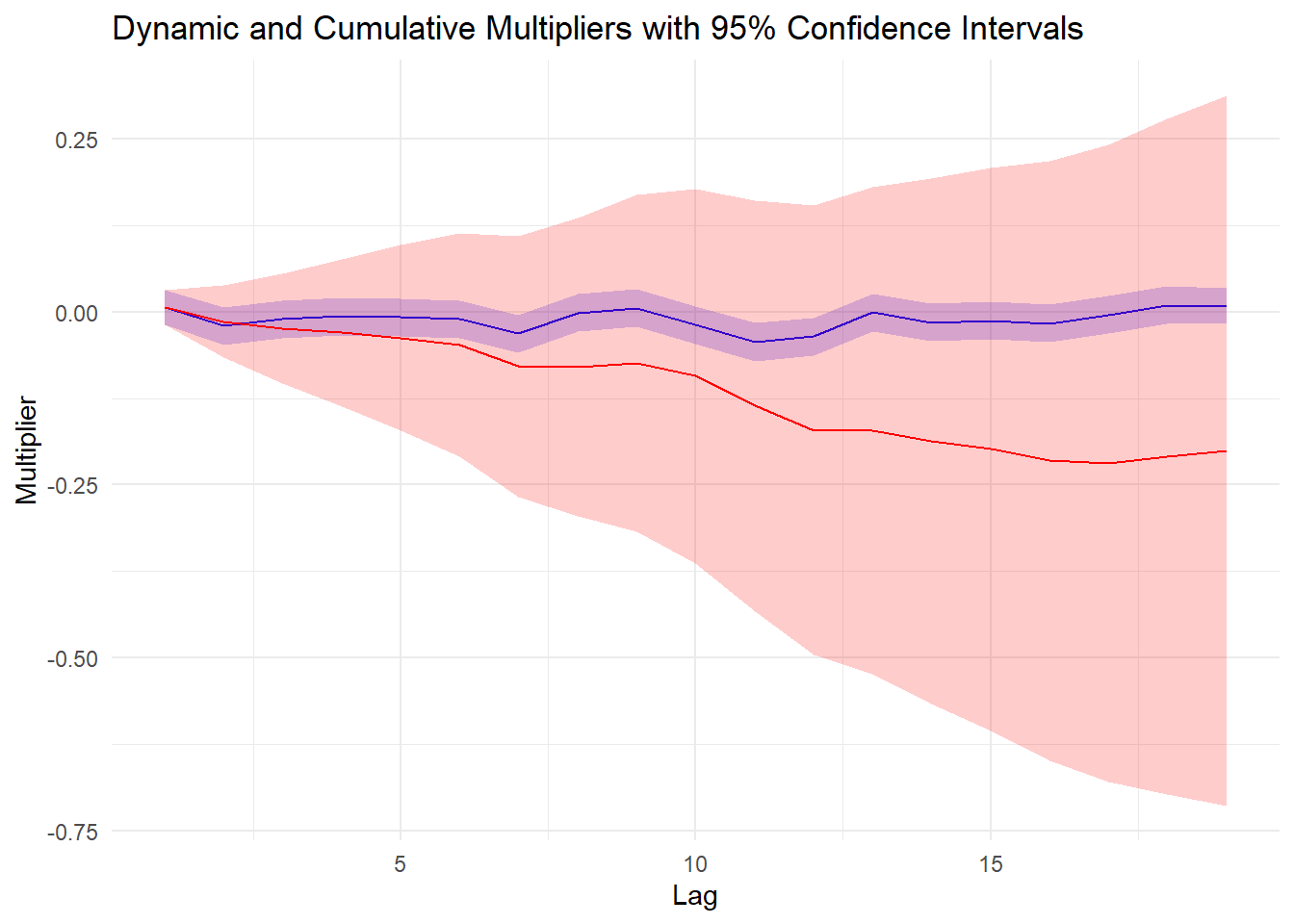
The values of dynamic are small. It indicates that the effect of 0_T on ip_growth is relatively weak.
f.
If high demand in the United States (evidenced by large values of ip_growth) leads to increases in oil prices, then 0_T is not exogenous. Exogeneity implies that the variable is not influenced by other variables in the model. In this case, if ip_growth affects 0_T, then 0_T is endogenous. The violation of the exogeneity assumption can lead to biased and inconsistent estimates of the coefficients in the distributed lag model. Consequently, the estimated multipliers shown in the graphs in part (e) may not be reliable. The presence of endogeneity can cause the estimated effects of 0_T on ip_growth to be either overestimated or underestimated.